Putting It All Together#

Overview

Teaching: 45 mins

Exercises: 10 mins

Questions:

Objectives: Create a simple research workflow using AWS EC2, AWS s3 and the AWS CLI

AWS CLI and EC2#

Now we will exit the CloudShell and explore a different way to access your virtual machines with the AWS CLI.

Let’s navigate back to the EC2 console. We can do this by navigating to the bento menu icon at the top of the navigation bar.

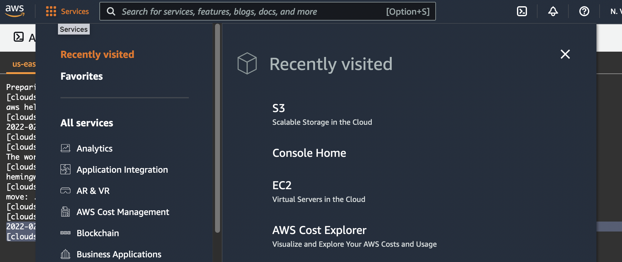
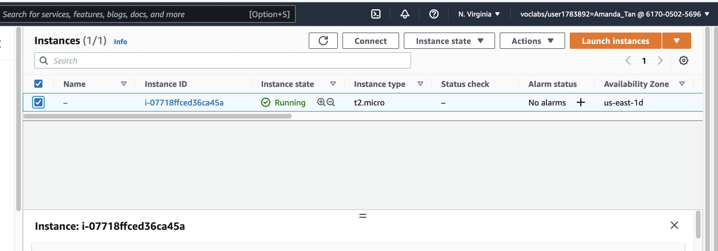
Once you are on the EC2 console, select your instance by clicking on the checkbox. The Connect button is at the top of the screen. Click on the connect button.

That should bring you to a page that looks something like this:

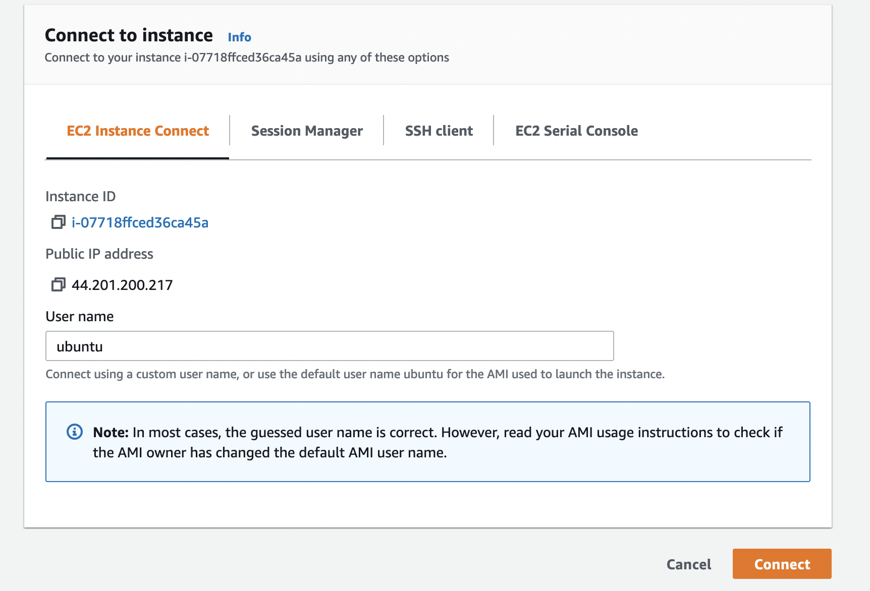
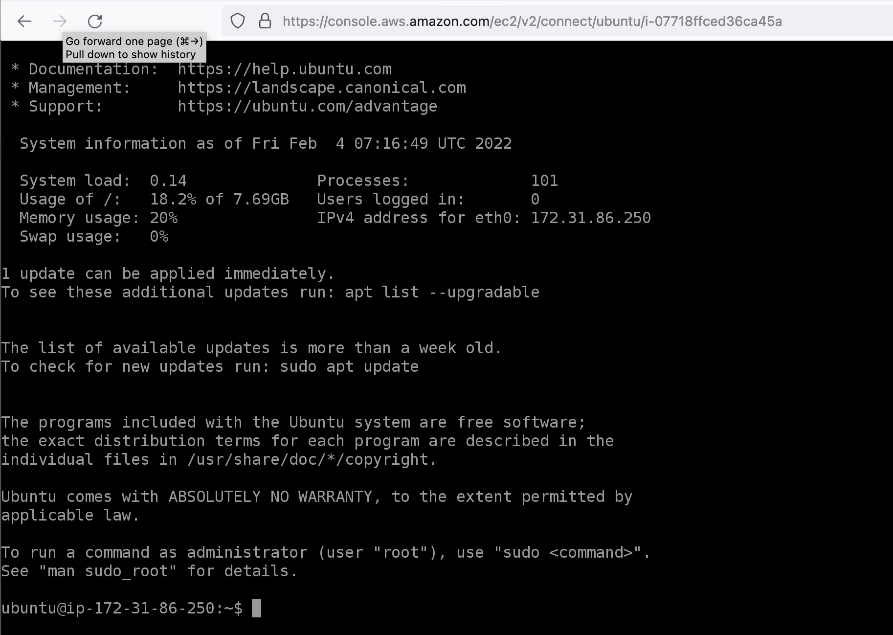
When you click connect, you will be connected to your EC2 instance via a secure shell tunnel!

Note

SSH or Secure Shell is a network communication protocol that enables two computers to communicate and share data.

Your virtual machine does not come pre-loaded with bells and whistles, so the first order business is making sure that it has the tools it needs for us to do some fun stuff. We will get the necessary updates and upgrades for the operating system.

sudo apt update | sudo apt upgrade

You will be prompted to install a whole slew of packages. Go ahead and press Y if prompted. This process may take a few minutes.

Next, we will install the aws cli package. Again, you will be prompted for installation. Press Y when prompted.

sudo apt  install awscli

Once the installation is complete, we can start linking together everything we have learn from the last few episodes. Recall that Drew needs to learn how to retrieve data from a cloud bucket, store the data and run some analysis on it.

Get example code onto EC2 instance#

Recall again that Drew needs to run some analysis on the dataset. We will first attempt to download our code to our EC2 instance. We will be downloading the code from a repository hosted in the cloud using the git command.

Note

Git is a version control system that lets you manage and keep track of your source code history. GitHub is a cloud-based hosting service that lets you manage Git repositories.

First check that git is installed:

git --version

git version 2.25.1

Now we’ll use git to “clone” a repository (i.e. copy the repository) from Github:

git clone https://github.internet2.edu/CLASS/CLASS-Examples.git

Cloning into ‘CLASS-Examples’…
remote: Enumerating objects: 66, done.
remote: Total 66 (delta 0), reused 0 (delta 0), pack-reused 66
Unpacking objects: 100% (66/66), 9.44 KiB | 508.00 KiB/s, done.

We now change the current directory to the Landsat directory in the CLASS-Examples directory that was just created by the previous git command and list the contents of the directory.

cd ~/CLASS-Examples/aws-landsat/ | ls -l

Public s3 buckets#

The data that Drew wants to work with is from the Landsat 8 satellite. The Landsat series of satellites has produced the longest, continuous record of Earth’s land surface as seen from space.The bucket that Drew wants to obtain data from is part of the AWS Open Data program. The Registry of Open Data on AWS makes it easy to find datasets made publicly available through AWS services. Drew already knows that the data exists in a public s3 bucket at s3://landsat-pds. Public in this case means that anyone can freely download data from this bucket.

Let’s look at what is stored in the s3://landsat-pds bucket.

aws s3 ls s3://landsat-pds

You should see a list of files and folders that are hosted on the s3://landsat-pdsbucket. More information about this bucket and its related files and folders can be found here: https://docs.opendata.aws/landsat-pds/readme.html.

We can also list the contents of a folder in the bucket.

aws s3 ls s3://landsat-pds/c1/

                       PRE L8/

You will now notice that there is A LOT of data in this bucket. In fact, a single Landsat8 scene is about 1 Gb in size since it contains a large array of data for each imagery band and there is almost a Petabyte of data in this bucket and and growing!

Note

Downloading data from one bucket to another is not a recommended practice when working on the cloud. Ideally, you would develop a workflow that allows you to bring your compute to the cloud instead of transferring data. Several new data formats like Cloud-Optimized Geotiffs (COGs) allow you to work directly with cloud-hosted data instead of having to download data.

We will test how to extract the data one for one Landsat8 image (scene). The area that our resident scientist, Drew is interested in is located in the Sierra Nevada mountains. From this converter: https://landsat.usgs.gov/landsat_acq#convertPathRow, Drew has determined that he would like to work with a scene from path 42, row 34 or latitute 37.478, longitude -119.048. He would also like to with the Landsat8 Collection 1 data, Tier 1 data for the dates of June 16 - June 29, 2017 due to low cloud cover for this dataset.

Let’s list the files that are in the s3 bucket that contains all these parameters. Each of these files contains an image for a particular spectral band. :

aws s3 ls s3://landsat-pds/c1/L8/042/034/LC08_L1TP_042034_20170616_20170629_01_T1/

Running an Analysis#

We will now use the process_sat.py script to open the files in this s3 bucket and run some analysis using an open-source package called rasterio.

Let’s first install the package:

sudo apt-get install python3-rasterio --yes

After installation, we can check our working directory and list the directory content. Make sure you are in the folder ~/CLASS-Examples/aws-landsat/

pwd

/home/ubuntu/CLASS-Examples/aws-landsat/

Let’s take a look at process_sat.py

cat process_sat.py

#!/usr/bin/python3
import os
import rasterio
import numpy as np

print('Landsat on AWS:')
filepath = 'https://landsat-pds.s3.amazonaws.com/c1/L8/042/034/LC08_L1TP_042034_20170616_20170629_01_T1/LC08_L1TP_042034_20170616_20170629_01_T1_B4.TIF'
with rasterio.open(filepath) as src:
    print(src.profile)

with rasterio.open(filepath) as src:
   oviews = src.overviews(1) # list of overviews from biggest to smallest
   oview = oviews[-1] # let's look at the smallest thumbnail
   print('Decimation factor= {}'.format(oview))
   # NOTE this is using a 'decimated read' (http://rasterio.readthedocs.io/en/latest/topics/resampling.html)
   thumbnail = src.read(1, out_shape=(1, int(src.height // oview), int(src.width // oview)))

print('array type: ',type(thumbnail))
print(thumbnail)

date = '2017-06-16'
url = 'https://landsat-pds.s3.amazonaws.com/c1/L8/042/034/LC08_L1TP_042034_20170616_20170629_01_T1/'
redband = 'LC08_L1TP_042034_20170616_20170629_01_T1_B{}.TIF'.format(4)
nirband = 'LC08_L1TP_042034_20170616_20170629_01_T1_B{}.TIF'.format(5)

with rasterio.open(url+redband) as src:
    profile = src.profile
    oviews = src.overviews(1) # list of overviews from biggest to smallest
    oview = oviews[1]  # Use second-highest resolution overview
    print('Decimation factor= {}'.format(oview))
    red = src.read(1, out_shape=(1, int(src.height // oview), int(src.width // oview)))
    print(red)
    
with rasterio.open(url+nirband) as src:
    oviews = src.overviews(1) # list of overviews from biggest to smallest
    oview = oviews[1]  # Use second-highest resolution overview
    nir = src.read(1, out_shape=(1, int(src.height // oview), int(src.width // oview)))
    print(nir)

def calc_ndvi(nir,red):
    '''Calculate NDVI from integer arrays'''
    nir = nir.astype('f4')
    red = red.astype('f4')
    ndvi = (nir - red) / (nir + red)
    return ndvi

np.seterr(invalid='ignore')
ndvi = calc_ndvi(nir,red)
print(ndvi)

localname = 'LC08_L1TP_042034_20170616_20170629_01_T1_NDVI_OVIEW.tif'

with rasterio.open(url+nirband) as src:
    profile = src.profile.copy()

    aff = src.transform
    newaff = rasterio.Affine(aff.a * oview, aff.b, aff.c,
                             aff.d, aff.e * oview, aff.f)
    profile.update({
            'dtype': 'float32',
            'height': ndvi.shape[0],
            'width': ndvi.shape[1],
            'transform': newaff})  

    with rasterio.open(localname, 'w', **profile) as dst:
        dst.write_band(1, ndvi)
     

We see that in ‘process_sat.py’ we will be opening the Red and Near Infrared band overview files using rasterio, then calcuting the Normalized Difference Vegetation Index (NDVI) which is a measure of changes in vegetation or landcover.

Let’s run process_sat.py:

./process_sat.py

Landsat on AWS: {‘driver’: ‘GTiff’, ‘dtype’: ‘uint16’, ‘nodata’: None, ‘width’: 7821, ‘height’: 7951, ‘count’: 1, ‘crs’: CRS.from_epsg(32611), ‘transform’: Affine(30.0, 0.0, 204285.0, 0.0, -30.0, 4268115.0), ‘blockxsize’: 512, ‘blockysize’: 512, ‘tiled’: True, ‘compress’: ‘deflate’, ‘interleave’: ‘band’} Decimation factor= 81 array type: <class ‘numpy.ndarray’> [[0 0 0 … 0 0 0] [0 0 0 … 0 0 0] [0 0 0 … 0 0 0] … [0 0 0 … 0 0 0] [0 0 0 … 0 0 0] [0 0 0 … 0 0 0]] Decimation factor= 9 [[0 0 0 … 0 0 0] [0 0 0 … 0 0 0] [0 0 0 … 0 0 0] … [0 0 0 … 0 0 0] [0 0 0 … 0 0 0] [0 0 0 … 0 0 0]] [[nan nan nan … nan nan nan] [nan nan nan … nan nan nan] [nan nan nan … nan nan nan] … [nan nan nan … nan nan nan] [nan nan nan … nan nan nan] [nan nan nan … nan nan nan]]

Let’s check if we obtained an image in our directory:

ls

LC08_L1TP_042034_20170616_20170629_01_T1_NDVI_OVIEW.tif process_sat.py

Now we need to upload this image to our s3 bucket.

Exercise

How would you find the name of your s3 bucket and copy the file LC08_L1TP_042034_20170616_20170629_01_T1_NDVI_OVIEW.tif over?

Once we have uploaded the image, we can check if it’s in the bucket:

aws s3 ls s3://bucket-userXXXXXXX

2022-02-08 05:51:01 1837900 LC08_L1TP_042034_20170616_20170629_01_T1_NDVI_OVIEW.tif
2022-02-04 06:45:30 26 hemingway.txt

Internet2 Cloud Learning And Skills Sessions

Putting It All Together

Contents

Putting It All Together#

AWS CLI and EC2#

Get example code onto EC2 instance#

Public s3 buckets#

Running an Analysis#